Performing Automated Critical Turner Rate Calculations with OnPing
I often see interesting equations on the whiteboards of Petroleum Engineers when I visit their offices. Recently, I overheard someone discussing an app to calculate an Automated Critical Turner Rate. This rate is used to determine if a gas well is experiencing liquid loading. It’s a straightforward calculation, and you can work through it pretty quickly.
But what if you wanted to bring it online and have a continually calculating critical rate based on changing bottom-hole pressures and temperature conditions? This seemed like a fun challenge to code in Inferno, using OnPing’s virtual parameters.
First, I need a solid reference implementation. I’m going to use Peng Tools’ liquid loading page as my reference example. The explanation there is well organized, but I will expand on each piece in the context of transforming it into an online calculation with several configuration options.
What is liquid loading?
When gas is produced in a well, liquids like water and condensate are also produced. If enough liquid accumulates, it can trap the gas. Ideally, the liquid flows up the walls of the tubing while the gas flows through the center. This situation, known as annular flow, causes the liquid to alternate between a film along the tube’s walls and small droplets. The fundamental concept behind the Turner Rate is that there is a minimum mass flow rate required to keep droplets from accumulating. The Turner Rate has been refined over the years, but we will focus on a version close to the original, using some of the adjusted constants employed by Peng Tools.
TL;DR:
If you already use OnPing, this script enables you to build an online version of an Automated Critical Turner Rate calculation immediately!
Required Parameters:
- \( P_{wf} \): Bottom Hole Flowing Pressure (psiA)
- \( T_{wf} \): Bottom Hole Flowing Temperature (°R)
- \( \sigma \): Water Surface Tension (dyne/cm)
- \( \rho_g \): Gas Density (lb/ft³)
- \( SG_g \): Gas Specific Gravity
- \( \rho_L \): Liquid Density (lb/ft³)
- \( d_{id} \): Tubing Internal Diameter (in)
- \( z \): Gas Compressibility
Governing Equations
We’ll build from the bottom up, starting with the critical rate equation:
Critical Rate Equation
\[ Q_g = 3.067 \frac{P_{wf} \cdot v_g \cdot A}{T_{wf} \cdot z} \]
- \( Q_g \): Gas Flow Rate
- 3.067: Empirical constant obtained experimentally
- \( P_{wf} \): Bottom Hole Flowing Pressure
- \( v_g \): Gas Velocity
- \( A \): Flow Area of the Tube
- \( T_{wf} \): Bottom Hole Flowing Temperature in Rankine
- \( z \): Gas Compressibility
This equation includes a few sub-equations for \( v_g \), temperature conversion to Rankine \( T_R \), and the tube flow area \( A \).
Temperature Conversion
Convert temperature from Fahrenheit to Rankine:
\[ T_R = T_F + 459.67 \]
Area of the Tube
To get the area \( A \) of the tube from its internal diameter \( d_{id} \):
\[ A = \frac{\pi d_{id}^2}{4} \]
Velocity Equation
The gas velocity \( v_g \) is defined as:
\[ v_g = 1.593 \left(\frac{\rho_L – \rho_g}{\rho_g}\right)^{1/4} \]
- \( v_g \): Gas velocity
- \( \rho_L \): Liquid Density
- \( \rho_g \): Gas Density
- 1.593: Empirical constant from experimental data
This equation implies that as liquid density \( \rho_L \) increases, a higher gas velocity \( v_g \) is needed to prevent liquid loading.
Gas Density Calculation
Finally, to calculate gas density \( \rho_g \):
\[ \rho_g = \frac{M_{air} \cdot SG_g \cdot P_{wf}}{z \cdot R \cdot T_{wf}} \]
- \( M_{air} \): Molar mass of air
- \( SG_g \): Gas Specific Gravity
- \( P_{wf} \): Bottom Hole Flowing Pressure
- \( z \): Gas Compressibility
- \( R \): Ideal Gas Constant
- \( T_{wf} \): Bottom Hole Flowing Temperature in Rankine
This setup includes all necessary components to set up an Automated Critical Turner Rate calculation for gas wells experiencing liquid loading.
OnPing Calculation Setup
We have everything we need to start building our calculation in OnPing. We’re going to create a set of manual parameters using test data from Peng.
Manual Parameters (Test Data)
- Bottom Hole Flowing Pressure (psiA): 400
- Bottom Hole Flowing Temperature (°F): 120
- Water Surface Tension (dyne/cm): 60
- Specific Gravity: 0.6
- Gas Compressibility: 0.9
- Tubing Internal Diameter (in): 1.995
- Liquid Density (lb/ft³): 67
Let’s Start Calculating!
With these parameters set up, we’re ready to run the calculation step-by-step in OnPing.
Area first…
        let area =
        Option.map
          (fun d -> let ft = d / 12.0 in pi / 4.0 * ft * ft)
          (latestValue tubing_diameter)
The map function allows us to convert the tubing diameter to area without checking if it exists.
We need to convert the temperature to degrees R.
let convertToRankine = fun T -> T + 459.67 in
Compute Gas Density
The formula for gas density \( g \) is:
\[
g = \frac{M_{air} \cdot SG_g \cdot P_{wf}}{z \cdot R \cdot T_{wf}}
\]
This becomes the following code:
        let computeGasDensity =
        fun p t z sg ->
            let airMass = 28.967 in
            let R = 10.732 in
            (airMass * sg * p) / (R * z * t)
Here, airMass and R are constants embedded in the function.
Compute Gas Velocity
Now that we have a function to calculate gas density, we need one for gas velocity:
The formula for gas velocity \( v_g \) is:
\[
v_g = 1.593 \cdot \left(\sigma^{\frac{1}{4}}\right) \cdot \left(\rho_L – \rho_g\right)^{\frac{1}{4}} \div \rho_g^{\frac{1}{2}}
\]
This becomes the following code:
        let computeGasVelocity =
        fun sigma rhoL rhoG ->
            let ef = 1.593 in
            ef * (sigma ** (1 / 4)) * (rhoL - rhoG) ** (1 / 4) / (rhoG ** (1 / 2))
In this code:
-
**means “to the power of” -
efstands for “engineering factor” and could be expanded for clarity.
Note that this equation shows we need to compute g (gas density) and provide l (liquid density).
Compute Critical Rate
Finally, we’re ready to compute the critical rate:
The formula for critical rate \( Q_g \) is:
\[
Q_g = 3.067 \cdot \frac{P_{wf} \cdot v_g \cdot A}{T_{wf} \cdot z}
\]
This becomes the following code:
        let computeCriticalRate =
        fun p v A z t ->
            let ef = 3.067 in
            ef * (p * v * A) / (t * z)
By embedding everything as functions, we create a straightforward correspondence with the paper and source material. Now, we need to apply these functions to OnPing data.
Using Pattern Matching with OnPing Data
        match
          ( area
          , latestValue bhp
          , Option.map convertToRankine (latestValue bht)
          , latestValue tension
          , latestValue gravity
          , latestValue compressibility
          , latestValue tubing_diameter
          , latestValue liquid_density
          )
        with {
         | ( Some A
           , Some bhP
           , Some bhT
           , Some surfaceTension
           , Some specificGravity
           , Some z
           , Some tubingDiameter
           , Some rhoL )
         ->
           let rhoG = computeGasDensity bhP bhT z specificGravity in
           let gasVelocity = computeGasVelocity surfaceTension rhoL rhoG in
           let criticalRate = computeCriticalRate bhP gasVelocity A z bhT in
           Some criticalRate * 1000.0 // Transform from MMscf to Mscf.
         | _ -> None
Here:
- The
latestValuefunctions retrieve the most recent values in OnPing for each variable, returningSomeif a value is present andNoneif it’s not. - We use pattern matching to handle
Optionalvalues, capturing the potential absence of data without using multipleifstatements. If any values are missing, the calculation returnsNone. - The
**operator means “to the power of,” andefis the “engineering factor” embedded in the function for clarity. - We convert the result from MMscf to Mscf by multiplying by 1000.0, since most flow meters use Mscf.
The computed critical rate value matches the expected result of 578.36 after conversion!
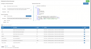
Here is the resulting Parameter.

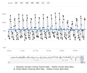
But the fun part comes when we swap out single calculations for downhole temperature and pressure with streaming variants! We can just reassign the variables a presto, we have our online calculation. Here is a trend of our critical turner rate against the flow rate for an example well.

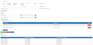
The turner rate fluctuates as does the flow rate. We might want to compare against the average flow rate to know if we are probably safe from loading. Using OnPing’s approximation capabilities let’s produce a report with a rolled up flow rate.

We can see the rolled up flow rate is 730.5 compared to our critical turner rate of around 630. It seems we are probably okay!
Conclusion
We hope this breakdown on creating an Automated Critical Turner Rate calculation in an online setting through OnPing has been helpful. Please let us know if you have any questions!

